Elasticsearch Guide

Ideas you will meet

Search

Inverted indexes, relevance, autocomplete and search engines.

Databases

Schemas, indexes, query plans and choosing a store.

What we already know about this

Our own lessons on these ideas. Read them here before you start, so it makes sense.

• Search, Analytics and Geo · 11 minSharding a search index: scatter, gather and mergeHow a search index is split across machines, why queries fan out to every shard, how top-k results are merged, and what goes wrong with deep paging and uneven shards.Read hereClose

  Why shard

  One machine cannot hold or search a very large index within the latency budget. Sharding splits the index into pieces, each on its own machine, so storage and work are spread out. Replicas copy each shard for availability and extra read capacity.

  Before: one big index

  100%

  After: sharded, scatter and gather

  100%

  What changed

  • Storage and work are spread over machines
  • Each shard returns its own top results to be merged
  • The slowest shard decides how fast the query is

  Two ways to partition

  • Document-partitioned (local index): each shard indexes a subset of the documents and holds a complete inverted index for them. Writes touch one shard. Every query must visit every shard. This is what Elasticsearch and Solr do.
  • Term-partitioned (global index): each shard holds the postings for a subset of terms. A query touches only the shards for its terms, but a write touches many shards and long posting lists must be combined across machines. It is rare in practice.

  100%

  Figure SDA-SAG-05-1 · Scatter, gather and merge · © forcsguy.com

  Decisions that matter

  • Shard size and count. Too many tiny shards waste memory and add fan-out; too few huge shards recover slowly and cannot spread load. Many teams aim for tens of gigabytes per shard. The primary shard count is hard to change later, so plan for growth or use time-based indexes.
  • Routing. By default a document goes to a shard by hashing its id, which spreads data evenly. Routing by tenant or user keeps one customer's data together so queries can hit a single shard, at the risk of uneven shards.
  • Tail latency. A query is as slow as its slowest shard. Use replicas, timeouts, and hedged requests (send to a second replica if the first is slow).
  • Deep pagination. Page N needs the first N x pageSize results from every shard. Use cursors (search-after) instead of large offsets.
  • Scoring across shards. Each shard computes statistics such as IDF from its own documents. Even, large shards make the difference small; otherwise gather global statistics first.
  • Rebalancing and reindexing. Plan how to add capacity without downtime, usually by indexing into a new index and switching an alias.

  100%

  Figure SDA-SAG-05-2 · Time-based indexes · © forcsguy.com

  Keeping the index fresh

  Documents usually live in a primary database and are copied to the search index. Use a change stream or an outbox so updates are not lost, accept that search is eventually consistent, and keep a way to rebuild the whole index from the source of truth.

  Real-world reading

  Related reading

  • Elasticsearch: scalability and resilienceElasticDocumentation
  • SolrCloud: shards and indexing dataApache Solr · Apache Software FoundationDocumentation
  • Elasticsearch GuideElasticDocumentation
  • Scaling Elasticsearch Clusters at UberUber engineers · UberCase Studies

  Show 2 moreShow fewer

  • Elasticsearch Performance Tuning Practice at eBayeBay engineers · eBayCase Studies
  • Solr: Improving Performance for Batch Indexing at BoxBox engineers · BoxCase Studies

  Open this lesson with its quiz and exercise

• Big Data and Cloud Data Platforms · 11 minHow big data evolved, and the papers behind itFrom single databases to Hadoop, Spark, streaming and lakehouses: a timeline of ideas and the research papers that started each one.Read hereClose

  Why a new wave kept appearing

  Each generation of data tools answered a limit of the previous one. Understanding the problem behind each wave makes the tools easier to place.

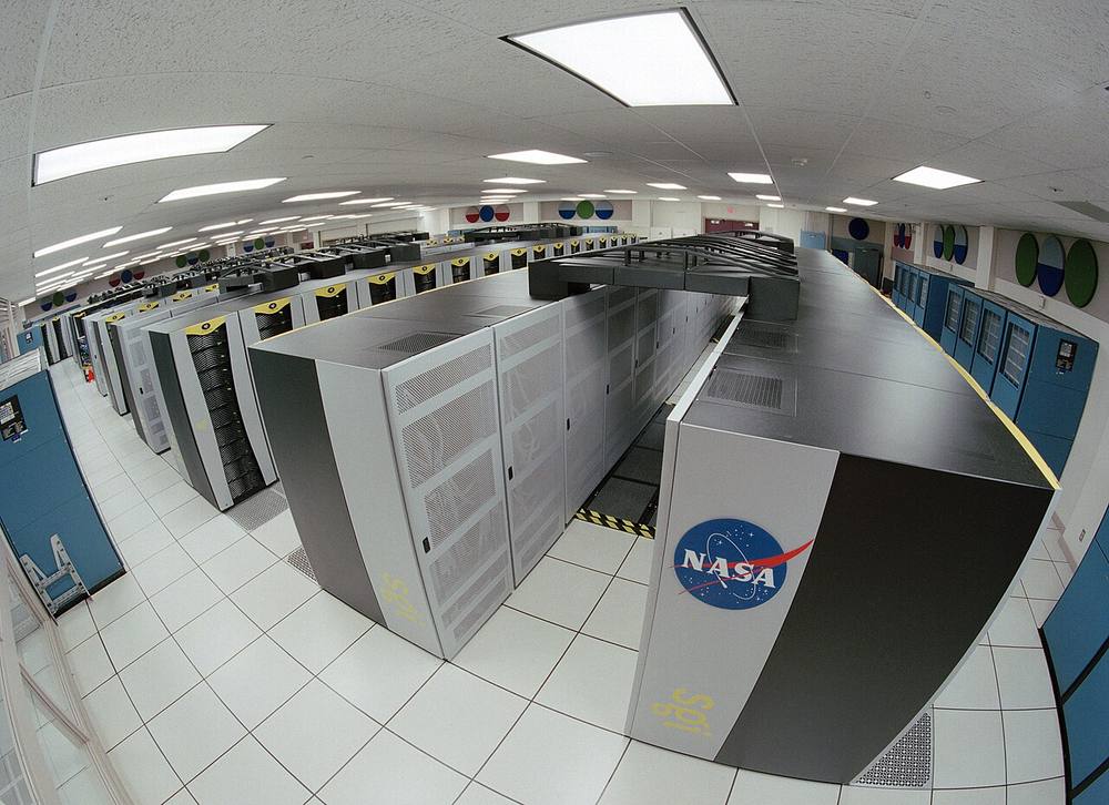  Image: Trower, NASA · Public domain · Source · Wikimedia Commons: Columbia Supercomputer - NASA Advanced Supercomputing Facility

  A timeline

  100%

  Figure SDA-BDP-01-1 · A timeline · © forcsguy.com

  1. Before: relational databases and data warehouses

  Data fit on one big server. SQL and data warehouses served reports. Limits: scaling up got very expensive, and unstructured data (web logs, clicks) did not fit neatly.

  2. Web scale (around 2003 to 2006)

  Search companies had far more data than any single machine could hold. Google described how it coped, and open-source projects copied the ideas.

  • GFS (Google File System): a distributed file system on commodity machines that expects failures.
  • MapReduce: a model to process huge datasets in parallel.
  • Hadoop (HDFS plus MapReduce) brought both to everyone.

  3. NoSQL (about 2006 to 2010)

  Web applications needed massive scale and high availability that relational systems struggled to give.

  • Bigtable: a sparse, sorted, wide-column store; inspired HBase and Cassandra's data model.
  • Dynamo: an always-writable key-value store with consistent hashing and eventual consistency; inspired Cassandra, Riak and DynamoDB.

  4. Faster and friendlier processing (2010 onward)

  • Dremel: interactive SQL over huge datasets using columnar storage and tree-shaped execution; the idea behind BigQuery and later engines, and the Parquet format.
  • Spark (resilient distributed datasets): keeps data in memory between steps, much faster than disk-based MapReduce for iterative work, with friendly APIs.

  5. Streaming

  Waiting for nightly batches was too slow. Kafka made a durable, replayable log the backbone of event pipelines, and engines such as Flink and the Dataflow model handled continuous computation with proper treatment of event time, windows and late data.

  6. The cloud

  Cloud providers separated storage (cheap object storage) from compute (elastic clusters or serverless queries). Managed warehouses (BigQuery, Redshift, Snowflake and others) removed cluster management.

  7. The lakehouse

  Data lakes were cheap but unreliable (no transactions, messy files). Table formats (Delta Lake, Apache Iceberg, Apache Hudi) add ACID transactions, schema evolution and time travel on top of files in object storage, so one copy of data can serve both analytics and machine learning.

  100%

  Figure SDA-BDP-01-2 · Key dates, in order · © forcsguy.com

  The classic papers

  These are the research papers most often cited. Search the title to find each; most are freely available.

  Paper	Authors (and year)	The idea
  The Google File System	Ghemawat, Gobioff, Leung (2003)	Large-file storage across commodity machines, built to tolerate failures
  MapReduce: Simplified Data Processing on Large Clusters	Dean, Ghemawat (2004)	A simple map and reduce model with automatic parallelism and fault tolerance
  Bigtable: A Distributed Storage System for Structured Data	Chang and others (2006)	A sorted, sparse, multi-dimensional map for structured data at scale
  Dynamo: Amazon's Highly Available Key-value Store	DeCandia and others (2007)	Consistent hashing, quorums, vector clocks and eventual consistency
  Dremel: Interactive Analysis of Web-Scale Datasets	Melnik and others (2010)	Columnar nested data and tree execution for fast SQL
  Kafka: a Distributed Messaging System for Log Processing	Kreps, Narkhede, Rao (2011)	A partitioned, replicated log as the backbone for event data
  Resilient Distributed Datasets (Spark)	Zaharia and others (2012)	In-memory, fault-tolerant parallel computing
  Spanner: Google's Globally-Distributed Database	Corbett and others (2012)	Strongly consistent, globally distributed SQL using synchronised clocks
  The Dataflow Model	Akidau and others (2015)	A unified model for batch and streaming with event time and windows
  Delta Lake: High-Performance ACID Table Storage over Cloud Object Stores	Armbrust and others (2020)	Transactional tables on object storage: the lakehouse idea

  A good companion is Jay Kreps's essay "The Log: What every software engineer should know about real-time data's unifying abstraction" (2013).

  What to take away

  • Scale-out on cheap machines (GFS, MapReduce) made big data practical.
  • Availability versus consistency choices (Dynamo, Bigtable, Spanner) shaped databases.
  • Columnar storage (Dremel, Parquet) made analytics fast.
  • Logs and streams (Kafka, dataflow) made data continuous.
  • Separating storage from compute and open table formats define today's platforms.

  Real-world reading

  Related reading

  • Dremel: Interactive Analysis of Web-Scale Datasets (paper)Melnik et al. · GooglePapers
  • Cassandra architecture overviewApache Cassandra · Apache Software FoundationDocumentation
  • Fast Order Search using Data Pipeline and Elasticsearch at YelpYelp engineers · YelpCase Studies
  • Apache CassandraApache Software Foundation · GitHubGitHub

  Show 6 moreShow fewer

  • Amazon S3 strong consistencyAmazon Web ServicesDocumentation
  • Sherpa: Distributed NoSQL Key-Value Store at YahooYahoo engineers · YahooCase Studies
  • Elasticsearch GuideElasticDocumentation
  • MapReduce: Simplified Data Processing on Large Clusters (paper)Dean and Ghemawat · GooglePapers
  • HBase at SalesforceSalesforce engineers · SalesforceCase Studies
  • Columnar DatabasesAmazon Web Services engineers · Amazon Web ServicesCase Studies

  Open this lesson with its quiz and exercise

• Search, Analytics and Geo · 11 minBM25: the ranking function behind most search enginesHow BM25 adds saturation and length normalisation to TF-IDF, what k1 and b control, and how to compute a score by hand.Read hereClose

  Two fixes to TF-IDF

  BM25 ("best matching 25") keeps the idea of weighting rare terms, and adds two corrections:

  1. Saturation: the first few occurrences of a term matter a lot; the twentieth barely matters.
  2. Length normalisation: a term appearing three times in a tweet means more than three times in a book.

  The formula

  For a query with terms q, the score of document D is the sum over terms of:

  IDF(q) x f(q,D) x (k1 + 1) / ( f(q,D) + k1 x (1 - b + b x |D| / avgdl) )

  • f(q,D) is how many times the term occurs in D.
  • |D| is the length of D and avgdl the average document length in the index.
  • k1 (about 1.2) sets how fast the term saturates.
  • b (about 0.75) sets how strongly length matters.
  • A common IDF is ln(1 + (N - n + 0.5) / (n + 0.5)), which never goes negative.

  100%

  Figure SDA-SAG-02-1 · What BM25 adds on top of IDF · © forcsguy.com

  A worked example

  With k1 = 1.2, b = 0.75 and a term appearing 3 times:

  • Average-length document: 3 x 2.2 / (3 + 1.2) = 1.57.
  • Twice the average length: 3 x 2.2 / (3 + 1.2 x 1.75) = 6.6 / 5.1 = 1.29.
  • Same document but the term appears 30 times at average length: 30 x 2.2 / (30 + 1.2) = 2.12, close to the ceiling of k1 + 1 = 2.2.

  So ten times as many occurrences is worth only 35 percent more. That is saturation.

  // Minimal BM25 term score, ready to use in a toy engine
  function bm25(f: number, len: number, avgLen: number, N: number, n: number, k1 = 1.2, b = 0.75) {
    const idf = Math.log(1 + (N - n + 0.5) / (n + 0.5));
    return idf * (f * (k1 + 1)) / (f + k1 * (1 - b + (b * len) / avgLen));
  }
  

  Tuning in practice

  • Start with the defaults; they work for general text.
  • Short fields such as titles often want a lower b (length matters less), while long bodies keep the default.
  • Fields have different value: a match in the title usually counts for more than in the body, so engines let you weight fields (BM25F style) or run separate fields and combine the scores.
  • BM25 is a first-stage ranker. Many systems retrieve a few hundred candidates with BM25 and re-rank them with a machine-learned model that also uses freshness, clicks and personalisation.
  • Measure changes with the metrics in the evaluation lesson; never tune by looking at three queries.

  100%

  Figure SDA-SAG-02-2 · Retrieval then re-ranking · © forcsguy.com

  Real-world reading

  Related reading

  • The Probabilistic Relevance Framework: BM25 and BeyondStephen Robertson and Hugo Zaragoza · City University of LondonPapers
  • Practical BM25, part 2: the BM25 algorithm and its variablesElasticBlogs
  • Lucene BM25SimilarityApache Lucene · Apache Software FoundationDocumentation
  • Elasticsearch GuideElasticDocumentation

  Show 1 moreShow fewer

  • Self-Ranking Search with Elasticsearch at WattpadWattpad engineers · WattpadCase Studies

  Open this lesson with its quiz and exercise